LSTM + GARCH + Regression: A Hybrid Model for Bangladesh’s Stock Market
Why we split stock prediction across three models (a stacked LSTM for price, GARCH for volatility, and a linear regression to combine them) and how that roughly halved the error.

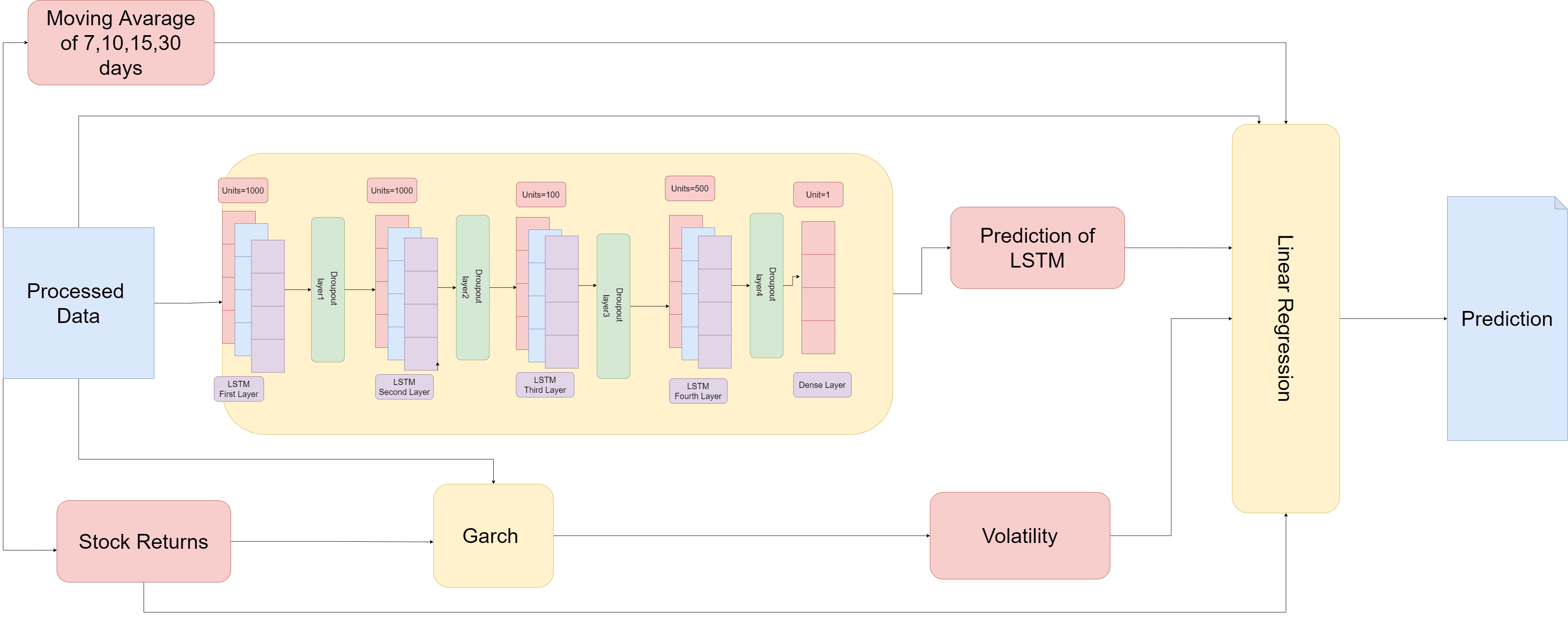
Table of contents
Most stock prediction tutorials use the S&P 500 or a handful of US tech stocks, where clean data is one API call away. We wanted to try the Dhaka Stock Exchange (DSE): a smaller, noisier emerging market with long flat stretches, sudden spikes and far less published research. This post covers how we built the hybrid model from our IEEE IEMCON 2022 paper, why we split the work across three models instead of one, and what the numbers showed.
The problem with one model
Stock prices carry two kinds of signal. One is the level and trend of the price, which a recurrent network like an LSTM can learn from recent history. The other is volatility: how wildly the price is swinging right now. Volatility clusters, so a calm week tends to follow a calm week and a turbulent one follows a turbulent one. Econometricians have modelled that for decades with GARCH.
An LSTM alone has to rediscover volatility from raw prices, and GARCH alone knows nothing about the price level. So we let each model do what it is good at and used a simple, interpretable linear regression to combine them.
Building the dataset
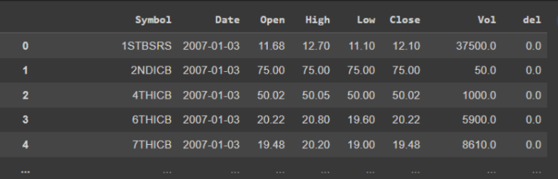
There was no ready-made DSE dataset, so we built one. AmarStock publishes one CSV file per trading day. We downloaded all 3,281 of them, covering 2007 to 2020, and merged them into a single file of 1,013,260 rows. Each row is one stock on one day: symbol, date, open, high, low, close and volume.
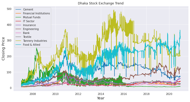
Cleaning was mostly routine: drop nulls, fix the date type, discard rows before January 2007, and pivot by ticker to find the most-traded stocks. Plotting closing prices by sector showed how differently each part of the market behaves, so we picked 11 stocks from different industries to test on: banks, telecom, fuel, pharma, ceramics, power and more.
Features
From the closing price we derived a small, deliberate set of features:
- Simple moving averages over 7, 10, 15, 20 and 30 days, to show the trend at several time scales.
- Daily percentage returns, (Cₜ − Cₜ₋₁) / Cₜ₋₁ × 100, plus log returns.
- The target, close_future: the close column shifted up by one row, so each row learns to predict the next day’s close.
The architecture
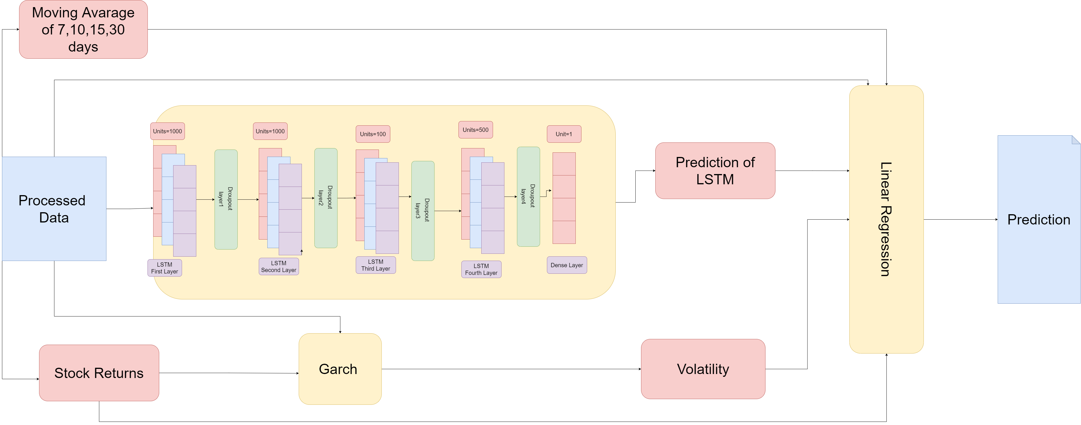
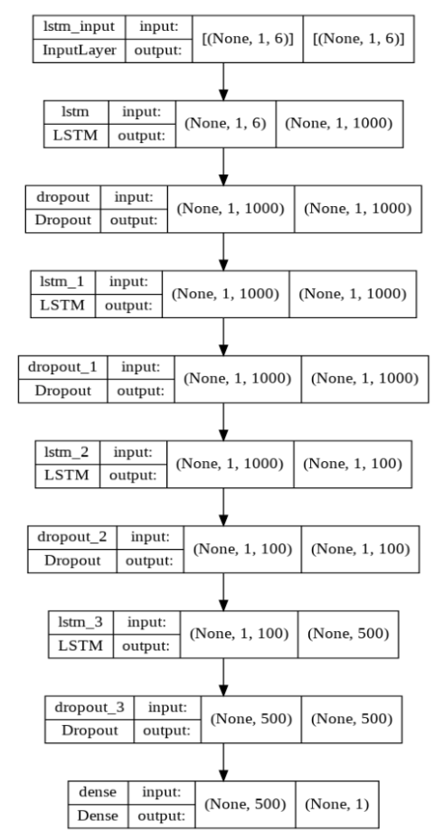
The model trains in three steps.
- Stacked LSTM. We split the data 80/20, scaled it to 0–1 with MinMaxScaler and built input windows with Keras’s TimeseriesGenerator. The network stacks four LSTM layers (1000, 1000, 100 and 500 units) with a 0.2 dropout layer after each, and ends in a single-unit dense layer.
- GARCH volatility. The autocorrelation of squared daily returns showed a strong spike at lag 9. To confirm, we fitted every GARCH(p, q) with p and q from 1 to 15 and kept the one with the lowest AIC, which was GARCH(9,13). On the test set it ran as a rolling one-day-ahead forecast, refitting as each new day arrived.
- Linear regression. The LSTM prediction, GARCH volatility, moving averages and returns go into a multiple linear regression, standardised with StandardScaler. Its coefficients show exactly how much weight each signal gets.
Results
We measured root mean squared error (RMSE) on the held-out test set for each of the 11 stocks, and compared the hybrid against its two main components run on their own.
| Stock | Linear Regression | Stacked LSTM | Hybrid |
|---|---|---|---|
| AB Bank | 0.57 | 1.48 | 0.12 |
| AMCL (PRAN) | 1.52 | 5.06 | 0.90 |
| Apex Tannery | 0.95 | 6.38 | 0.50 |
| BD Finance | 0.54 | 1.05 | 0.24 |
| Grameenphone | 2.30 | 11.68 | 1.40 |
| Padma Oil | 1.28 | 6.34 | 0.74 |
| Popular Life | 0.84 | 5.19 | 0.37 |
| Samorita | 1.05 | 2.76 | 0.35 |
| RAK Ceramics | 0.68 | 3.09 | 0.27 |
| GBB Power | 0.52 | 1.30 | 0.11 |
| Beximco | 0.22 | 3.36 | 0.42 |
| Mean | 0.95 | 4.34 | 0.49 |
The hybrid had the lowest error on 10 of the 11 stocks, and its mean RMSE was about half that of linear regression. The exception is Beximco, where plain linear regression (0.22) beat the hybrid (0.42). We think that is worth reporting rather than hiding: a simpler model can still win on a given stock.
The stacked LSTM on its own was the weakest model, especially on high-priced, volatile stocks like Grameenphone. Its predictions often sat visibly off the real price. Once its output became one input to the regression, next to volatility and trend, most of that error disappeared.
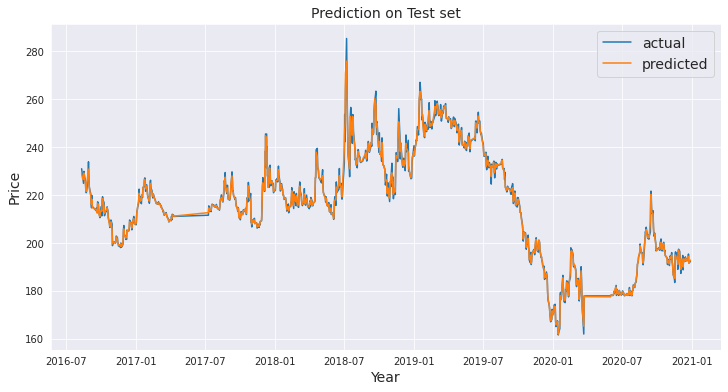
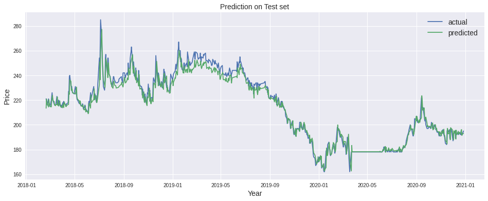
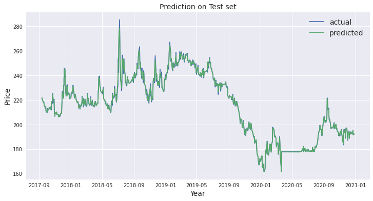
The same stock, AMCL (PRAN), through each model. The gap between the stacked LSTM’s prediction and the real price is easy to see; the hybrid follows the price much more closely.
What I’d do differently today
Looking back as an engineer, a few things would make these results more convincing:
- Walk-forward validation. A single 80/20 split is a start; rolling train/test windows show whether a model holds up across different market regimes.
- A naive baseline. For next-day prices, "tomorrow equals today" is surprisingly hard to beat. Every model should be measured against it.
- Directional accuracy. RMSE on price levels doesn’t say whether the model called up or down days correctly, which is what matters for a trading decision.
Takeaways
- Combining models works best when each one sees a genuinely different signal: trend, sequence and volatility.
- A linear regression makes a good final combiner. It is fast, stable and you can read off how much it trusts each input.
- Emerging markets like the DSE need you to build your own data pipeline, and cleaning the data is often the bigger half of the work.
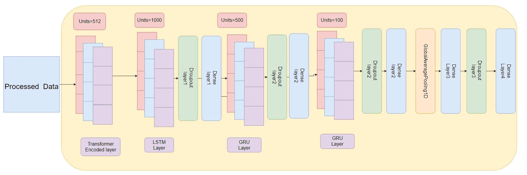
This work led to our follow-up paper, DeepDse, which swaps the LSTM for a Transformer–LSTM–GRU stack and adds gold, oil and USD prices as inputs.

Written by Omor Al Tanim
Newsletter
Enjoyed this? Get the next one by email
A short email when I publish something new on AI agents, ERP automation or research. No spam; unsubscribe in one click.
More from Omor Al Tanim
 In Research by Omor Al TanimSep 28, 2026Pinned
DeepDse: Predicting the Dhaka Stock Exchange with Transformers, LSTMs and GRUs
How we combined a Transformer encoder with LSTM and GRU layers, added gold, oil and USD prices as inputs, and got the lowest error on all 11 DSE stocks we tested.
- In AI/ML by Omor Al TanimJan 15, 2025
Building Multi-Agent Systems with Semantic Kernel
A deep dive into creating intelligent multi-agent systems using Microsoft Semantic Kernel for orchestrating complex AI workflows.
- In Engineering by Omor Al TanimJan 8, 2025
OCR Solutions for Document Processing
Exploring various OCR techniques and best practices for building robust document processing systems with Tesseract.
Comments (0)
Comments are checked by AI before they appear. Read the rules
Loading comments…